Foreword
Welcome!
This is the manual of AEON, a tool for long term analysis of Boolean networks. In particular, AEON allows you to define Boolean networks with partially unknown update functions. Then, for such a network, you can compute its asynchronous attractors and explore the state space of these attractors. Finally, you can investigate how the attractor structure changes depending on the unknown parts of the network (attractor bifurcation) as well as which variables are stable, unstable, or switched under different conditions (stability analysis). For all of this, AEON uses efficient symbolic algorithms based on BDDs, which make it possible to handle even networks with 1000 or more variables.
In this document, you can find information on how to use AEON to:
- Create a Boolean network or import it from an existing
.sbmlor.aeonfile. - Create a partially unknown Boolean network with logical parameters.
- Check that the network is consistent with its regulatory graph.
- Compute asynchronous attractors of a Boolean network.
- Visualize the state space of the computed attractors.
- Construct a bifurcation decision tree: A visual representation of the dependence between network parameters and attractors.
- Perform stability analysis of the attractors for different conditions.
AEON is a constantly evolving academic project. If you have any problem or run into some unexpected behaviour, please contact us at sybila@fi.muni.cz. We will be happy to help you and make AEON a more useful tool for you. Finally, if you found AEON useful in your research, please cite it using the following publication:
Beneš, N., Brim, L., Kadlecaj, J., Pastva, S., & Šafránek, D. (2020, July).
AEON: Attractor Bifurcation Analysis of Parametrised Boolean Networks.
In International Conference on Computer Aided Verification (pp. 569-581).
Introduction
AEON is available as an online tool at https://biodivine.fi.muni.cz/aeon/. On this website, you can pick the version of AEON you want to use (naturally, we recommend the latest version), and you will be redirected to its online interface, which should look similar to this:
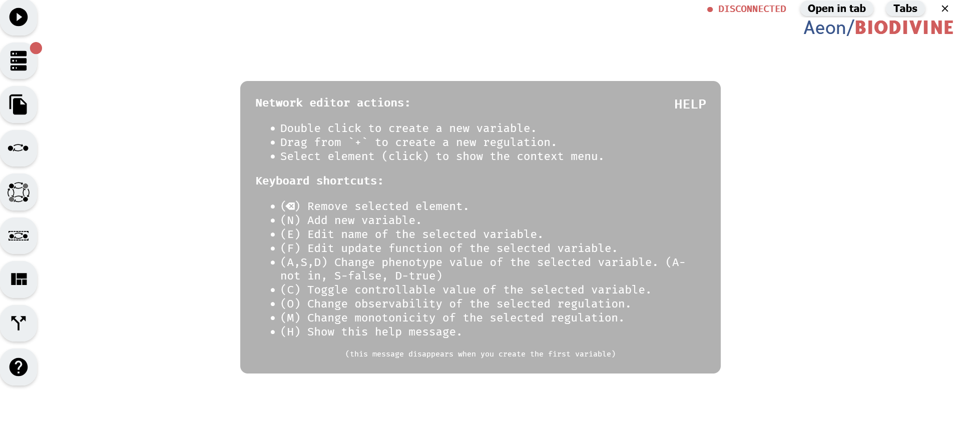 AEON User interface.
In the middle, there is a quick help message, which disappears when you load a Boolean network, but you can always bring it back by holding down H. On the left, there is a main menu which you can use to import existing networks, manage the details of your model, or start attractor analysis.
If you for whatever reason cannot access this website, there is a mirror on Github pages, but the version there may not be always up to date. Alternatively, you can also run your own instance of AEON. It is a simple static HTML/JavaScript website, and the sources are available on Github. See the Building AEON chapter for more details.
Out of the box, AEON allows you to perform basic actions, like creating or editing a Boolean network. However, AEON uses a native compute engine which handles computationally intensive tasks efficiently outside your browser. Therefore, to do almost anything beside editing Boolean networks, you need a compute engine the website can connect to. In the next chapter, we discuss how to download and run this compute engine.
At the moment, due to security reasons, some browsers are blocking non-HTTPS JavaScript connections to foreign websites if the page itself is using HTTPS. For this reason, you may not be able to connect to a local compute engine from Safari, Brave or other browser with this policy. If you can, please use Chrome for the rest of this tutorial.
AEON Compute Engine
To download the compute engine for the version of AEON you are using, pick Compute Engine in the left menu, and download a pre-compiled binary for your operating system. Compute engine binaries for different versions of AEON are in general not compatible, and you should be therefore always using the compute engine of your current version:
 Downloading AEON compute engine.
Once the download is finished, you can unzip the file. Inside, you should find a compute-engine binary that you need to execute.
The binary is not signed for distribution on MacOS, so you may need to add a security exception if you want to run it on a Mac.
When you execute the binary, you should see a terminal window with an output similar to this:
🔧 Configured for production.
    => address: localhost
    => port: 8000
    => log: critical
    => workers: 8
    => secret key: generated
    => limits: forms = 32KiB
    => keep-alive: 5s
    => read timeout: 5s
    => write timeout: 5s
    => tls: disabled
Warning: environment is 'production', but no `secret_key` is configured
🚀 Rocket has launched from http://localhost:8000
The compute engine automatically starts a local webserver on port 8000 through which it communicates with the AEON website. You can set the environmental variable AEON_PORT to whatever you need the port to be.
If you can't for any reason run the binary (for example, some Linux systems seem to have problems with outdated
glibc), you can build it from source. Instructions for this are quite simple, and you can find them in the Building AEON chapter.
Once compute engine is running, you can go back to the AEON website and either (a) refresh the website, if running correctly, the compute engine should connect automatically, or (b) press Connect in the Compute Engine panel to manually retry the connection. You should see the status change from disconnected to connected, and the dot next to the Compute Engine should change its color to green.
 Connecting to a running compute engine.
If you changed the
AEON_PORTvalue, you need to also update the engine address in theCompute Enginepanel — click the default addresshttp://localhost:8000to edit it.
WARNING: At the moment, the compute engine supports only one active session of AEON at a time (this will be resolved in future versions of AEON). If you have multiple tabs with AEON open, and they all connect to the same compute engine, they can see and override each other's data! You can still use multiple tabs to edit or view networks, but keep in mind that analysis results (attractors and bifurcation decision trees) are available only for the last computed tab.
Now, you should be ready to use all features available in AEON.
Model Editor
This chapter explains how to create, import, modify, and export Boolean networks in Aeon, along with enhancing them with logical parameters. If you only need to work with existing Boolean networks (available in .sbml or .aeon formats) without editing, you can skip to the final section of this chapter.
Aeon's model editing functionality is divided into two main components:
- Regulatory Graph Editor – The main area of the Aeon window, used for interactive editing of network structure.
- Model Panel – A sidebar that provides tools for modifying update functions and adding logical parameters. It can be opened by clicking the Model Editor button in the left menu.
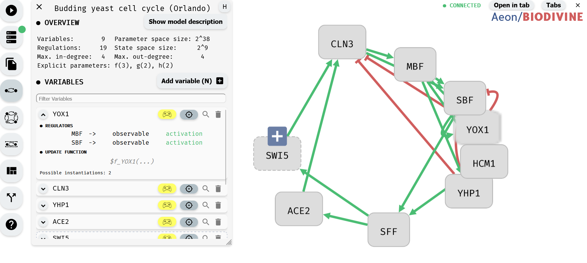 Model panel (left) and regulatory graph editor (right)
We first focus on the regulatory graph editor, and show how to manipulate network variables and regulations. Then, we shift our focus to the model panel and show how to edit network update functions or add parameters. Finally, we look at structural properties of regulatory graphs and how AEON verifies these properties on-the-fly. At the end of the chapter, we discuss model formats supported by AEON.
Note: This chapter does not cover setting control parameters with the Model Editor. For that, refer to the Setting of Control Parameters with Model Editor chapter
Variables and regulations
To create a new variable, double-click anywhere in the empty space of the AEON window. A new variable node will appear at that location (You can also press N to create a new variable node at a default location). A variable node in a regulatory graph represents one variable of a Boolean network. When you move the cursor over this variable node, a blue + icon appears. By dragging from this icon to some variable node, you can create regulations, i.e. edges of the regulatory graph. Note that self-loops (auto-regulations) are also supported. A regulation edge from A to B represents a (possible) dependence of B on A.
 Creating variables and regulations in the regulatory graph.
You can click and drag variable nodes to rearrange them freely within the network.
To assist with organizing large networks, Aeon provides an auto-layout algorithm that automatically arranges the nodes for better clarity. You can activate this feature using one of the Layout buttons in the Visual Options Module.
Additionally, the Visual Options Module allows you to highlight variable nodes based on their properties, making it easier to analyze specific aspects of the network.
 Auto-layout and highlight functionality.
Finally, each variable node or regulation edge can be selected by clicking. This opens a variable or regulation menu. Through here, you can access additional options, such as removing a variable or regulation (which you can do using backspace as well). You can also rename a variable, which opens the model panel and focuses the edit field of the variable name. We will talk about the remaining options in edge and regulation menus in the following sections.
 Deleting and editing regulatory graph elements.
Model panel and update functions
Once the regulatory graph of your Boolean network is in place, you can assign each variable an update function. The update function of variable A takes the values of its regulators (sources of the regulation edges terminating in A) and computes a new value of A based on these values.
For example, consider the following regulatory graph:
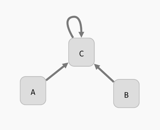
Here, variable C is regulated by every variable. That is, update function of C should depend on A, B, and C. For example, we can open the model panel and set the update function to C | (!A & !B). This will make C true if it already is true, or if both A and B are false.
 Setting the update function of
 C.
The behaviour of the Boolean network is described using a state transition graph, where the graph vertices are the states of the network (each state assigns true or false to every network variable), and the edges correspond to applications of individual update functions to the network states. In our network, a state A=false, B=false, C=false can transition into A=false, B=false, C=true by updating the variable C.
Note that A and B have no regulations, therefore their update functions do not depend on any variable and must be constant: true or false. In general, an update function can use the constant values true/false, names of the regulating variables, parenthesis (), and (&), or (|), implies (=>), if and only if (<=>) as well as xor (^). You can add new-lines and arbitrary whitespace to the update function, but AEON will not save this information to the exported model file.
Other model panel functionality
Aside from setting the update functions, in the model panel, you can create/remove variables as well as edit their names (as we have already seen). In a large model, it can be also useful to locate a specific variable in the regulatory graph using the magnifying glass button.
 Looking up and editing a variable in a model panel.
Hint: When the model is very large, you can use the "Find..." feature of your browser to look for specific variables in the model panel.
Finally, at the very top of the model panel, you can find an edit field where you specify the name of your model, as well as some general description of the model. This part of the panel also contains a general overview of the model, including:
- Number of Boolean variables and regulations between them.
- Maximal in-degree and out-degree (number of incoming and outgoing regulations) in the model.
- Size of the models state space.
- Size of the parameter space, as well as names of the logical parameters.
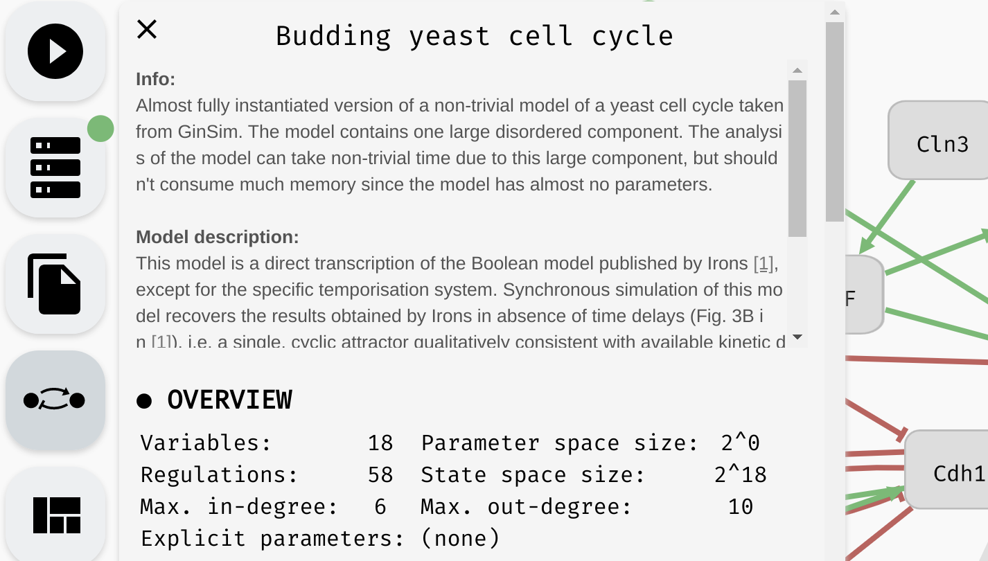 The name, description, and overview of a particular model.
Parametrised networks
In practice, we often don't know the exact update functions that govern the behaviour of the network. In AEON, you can therefore analyse even a network that is partially unknown. In such case, we say that the network has logical parameters. These parameters can be of two types:
- We say that a variable is implicitly parametrised when its entire update function is unknown. For example, in the model from the previous section, since we did not set any update function for
AorB, they are both implicitly parametrised. - An update function is explicitly parametrised when it contains unknown Boolean expressions. These are expressed using uninterpreted functions. For example, in the model from the previous section, we could set the update function of
Cto beC | f(A, B). Here,fis an explicit parameter: an uninterpreted function of arity 2. This way, we are giving a partial specification of the update function: we know that whenC=true, the value of the function is alsotrue. However, ifC=false, we know the result depends onAandB, but we don't know what that dependence looks like.
An uninterpreted function of arity zero can be also used without argument parenthesis, in which case it resembles a more traditional logical parameter. For example, we can write
(K => A) & (!K => B)whereAandBare variables, butKis an explicit parameter.
At the moment AEON only allows variables as arguments of uninterpreted functions. That is, you cannot use complex expressions such as
C | f(A & B, C). This restriction may be lifted in the future.
In AEON, we then consider all possible instantiations of these logical parameters. That is, AEON considers every possible Boolean function that can be substituted in place of either the explicit or implicit uninterpreted functions.
Note that the number of such functions grows very quickly (there are
2^(2^n)Boolean functions withnarguments). For this reason, AEON typically cannot handle uninterpreted functions (explicit or implicit) with more than 5 arguments (which corresponds to2^32possible functions).
In the user interface, you can see this in the form of Possible instantiations: ... label under each update function input field. If the function is fully specified (no parameters), there should be one instantiation: the function itself. As soon as parameters are introduced (or the function is removed completely), the number of instantiations should grow.
For example, update functions for variables A and B from our example should have two instantiations (true and false), while the C | f(A, B) function will have 10 instantiations, as there are 10 binary Boolean functions that depend on both inputs (There are 16 binary Boolean functions, but 6 of them, true, false, A, !A, B, and !B do not depend on both inputs).
Parameters will come into play later, when we discuss the long term behaviour of Boolean networks. Now, lets look at how we can reduce the number of possible instantiations of a parametrised network by enhancing the regulatory graph with additional structural properties.
Regulatory graph properties
In our regulatory graphs, to this point, we assumed each regulation should have some effect on the output of the update function. This is a fairly reasonable assumption (if the regulation has no effect, it has no reason to be in the graph). However, we often have some additional information about the nature of the regulation.
Regulation monotonicity
Many biological processes are either positively or negatively monotonous. In such case, we can mark a regulation as activation (positive monotonicity), or inhibition (negative monotonicity). To do this, you can either use the corresponding button in the regulation menu, or toggle the regulation status in the model panel.
 Changing monotonicity of regulations.
Notice that as we change the monotonicity of a regulation, the number of instantiations of the update function also changes. This is because the number of Boolean functions with that specific property is smaller. Specifically, if a regulation is positively monotonous, we expect that increasing the value of the regulator cannot decrease the value of the output, and vice versa, when the monotonicity is negative, increasing the value of the regulator cannot increase the function output.
Specifically, if we set the regulation B -> C as activation, we reduce the number of instantiations of f(A, B) to only four options: A & B, !A & B, A | B, !A | B. In particular, notice that in each such function, B appears in its positive form (without negation). We could further limit the number of instantiations by also setting a monotonicity for the A -> C relationship.
The regulation C -> C is slightly different. The dependence C -> C is already fully specified in the update function. Changing the properties of the regulation therefore cannot change the number of instantiations. However, it can make the function completely invalid if the properties given by the regulatory graph do not match the properties of the update function. Since in our case, C appears positively in C | f(A, B), AEON reports an error when the regulation is marked as an inhibition, but is ok with either activation or unspecified monotonicity.
When possible, AEON will try to infer which regulation properties cause the function to be invalid. You can then update the properties accordingly.
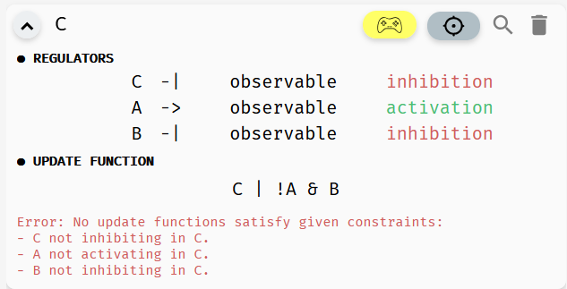 AEON explains why a function is not consistent with its regulatory graph.
Observability
While it is often reasonable to expect each regulation to have some effect on the regulated variable, sometimes we may not be sure if a regulation is indeed (always) needed. In such case, we can mark the regulation as non-observable.
AEON will then also consider instantiations where the argument does not have any impact on the resulting function value. To set this property, you can again use either the regulation menu, or the model panel:
 Changing observability of regulations.
Notice that as we remove the observability requirements, the number of instantiations grows. In the end, the function has 15 possible instantiations. This includes all 16 possible binary Boolean functions except for one: true.
If we set f(A, B) = true, the update function would be C | true, which is equivalent to true. However, we still have C -> C marked as observable, and a constant function does not depend on C. Meanwhile, instantiation f(A, B) = false is fine, because C | false is equivalent to C, which clearly still depends on the value of C.
Also, note that a function can "appear" to depend on a value of some variable, while in fact it does not. Take a simple example of (A & B) | A. If A=true, this function is always true, if A=false, this function is always false, regardless of the value of B. AEON will also detect and report these types of problems.
Inconsistencies in real world models
Note that in many cases, you can encounter real-world models where AEON identifies some structural inconsistencies as described in this section. In such case, you cannot directly analyse the original model.
This does not necessarily mean the model is incorrect, but it can suggest some kind of human error (a missing negation, wrong parenthesis, etc.), or an inconsistency between experimental data and literature (regulatory graph is often constructed based on known assumptions about the system, prior to the actual Boolean functions).
In such case, assuming you cannot consult the author(s) of the model about the inconsistency, we recommend simply updating the regulatory graph to make it consistent with the update functions in the model. That is, removing the monotonicity or observability requirement from the problematic regulation.
Import/Export
Finally, lets discuss how to transfer your models into AEON, as well as sharing them with the world afterwards. AEON has an Import/Export panel accessible in the left menu:
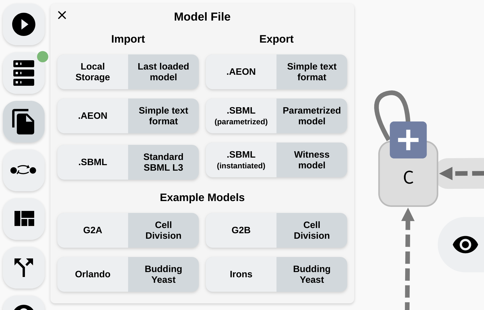 Import/Export panel in AEON.
At the bottom, you can see a collection of four pre-defined example models which you can open to demo AEONs functionality. Each model contains additional description of its properties.
The
Local Storageoption tries to continuously save the model you are working on into the local storage of your browser. If you accidentally reload your editor and lose some unfinished work, you can try to recover it from this local storage.
SBML-qual
AEON should be fully compatible with SBML-qual models. You can therefore both import and export .sbml models from AEON. However, there are a few restrictions to keep in mind:
- AEON only supports alphanumeric names with underscores, while SBML also supports other special characters (for example
[]). During import, AEON will replace all conflicting characters with underscores. If this leads to a name clash, it also adds a unique ID to the name of each variable. - AEON will try to import layout information from the SBML file, but the layout may be incompatible (some tools use a
[0,1]coordinate system, which makes the layout very small), or completely missing. In such case, all variable nodes will appear at the same position. You can then apply the automatic layout to better visualise the network. - SBML does not have explicit support for observability. If a regulator appears in an update function, AEON will import this regulation as observable. If the regulator is completely missing in the function, it will be imported as non-observable.
- SBML may contain variables with unspecified update functions. These are naturally imported as implicitly parametrised. However, there is no support for explicit parameters. To implement this functionality, if a model contains explicit parameters, we export the update function with a
<csymbol>MathML element (used to denote arbitrary function invocation). This can be imported back into AEON, but won't be interpretable in other tools that follow the SBML standard. You can disable this behaviour by using theSBML (instantiated)button. In this mode, AEON will pick some arbitrary instantiation for each parameter and thus export a valid SBML.
Aeon format
Since SBML is quite hard to edit by hand, as well as parse correctly, we also provide a simplified text based format. In this format, the regulatory graph is described as a list of edges, where each edge is encoded as regulator [->,-|,-?,->?,-|?,-??] target. Here, regulator and target are the names of the network variables, and the arrow connecting them describes the type of regulation. Then -> denotes activation, -| inhibition and -? is unspecified monotonicity. Finally, an extra ? signifies that the regulation is non-observable.
An update function for variable X is written as $A: function, where the format of the actual functions in .aeon files is the same as in the edit fields in the AEON interface. Additional information (model name, description and layout) is encoded in comments (lines starting with #). The order of declarations is not taken into account. Example of .aeon model:
    #name:Asymmetric Cell Division A
    #description:Lorem Ipsum....
    #position:CtrA:419,94
    CtrA -> CtrA
    GcrA -> CtrA
    CcrM -| CtrA
    SciP -| CtrA
    $CtrA: CtrA & GcrA & !CcrM & !SciP
    #position:GcrA:325,135
    CtrA -| GcrA
    DnaA -> GcrA
    $GcrA: !CtrA | DnaA
    #position:CcrM:462,222
    CtrA -> CcrM
    CcrM -| CcrM
    SciP -| CcrM
    $CcrM: CtrA | f(CcrM, SciP)
    #position:SciP:506,133
    CtrA -> SciP
    DnaA -| SciP
    #position:DnaA:374,224
    CtrA -> DnaA
    GcrA -| DnaA
    DnaA -| DnaA
    CcrM -> DnaA
    $DnaA: g(CtrA, GcrA, DnaA) & CcrM
Note that due to this encoding,
.aeontechnically can't represent a variable with no incoming or outgoing regulations. Such variable may be lost during export.
Attractor Bifurcation
In this chapter, you will learn how to study the long term behaviour of Boolean networks using AEON. Specifically, we refer to this analysis as attractor bifurcation, because it examines how parameters influence the long term behaviour (attractors) of a particular Boolean network.
Attractors are subgraphs of the asynchronous state transition graph of the Boolean network. Recall that this graph consists of states which assign Boolean value to each variable of the network, and transitions which correspond to applications of individual update functions. Then, attractor consists of states that, once reached, cannot be escaped. Informally, these are the regions where the network eventually converges to, and stays forever. In terms of graph theory, these are the bottom (terminal) strongly connected components of the state transition graph.
In AEON, we distinguish between three main types of attractors:
- Stable attractor is an attractor which consists of a single state. This type of attractor is also called a sink.
- Oscillating attractor is a cycle of states. The length of the cycle is its period, hence this type of attractor is sometimes also referred to as periodic.
- Disordered attractor is an arbitrary set of states consisting of multiple connected cycles. This type of attractor is also called aperiodic.
 Three types of attractors. Notice that each type is labelled with an appropriate icon.
To compute the attractors of the network, click Start Analysis in the left menu. Keep in mind that for large models (especially with a lot of parameters), this process can take a long time. The compute engine color should change to orange, and you should find a (very) approximate progress of the computation in the compute engine panel. Here, you can also cancel the current computation.
 Starting and cancelling a computation.
Due to the nature of the problem, it is typically not possible to accurately predict how long it will take to compute the results. The progress corresponds to the number of states eliminated as "non-attractor" states so far, however, this is only meaningful when the attractors are relatively small. Also, as discussed previously, AEON compute engine can only run one computation at a time. If you need to run multiple experiments simultaneously, we recommend running multiple compute engines.
Once the computation is finished, you should be taken to the Results panel, where you can see the overview of the attractor bifurcation function. If your model has no parameters, the function has one row showing the types of attractors in your network (behaviour class). In a parametrised model, there are usually multiple rows, each showing you the number of parametrisations (witness count) which produce a specific type of behaviour.
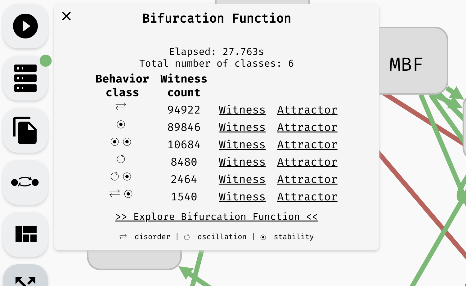 An overview of an attractor bifurcation function of a parametrised Boolean network. There are 6 behaviour classes, two having an oscillating attractor and two having a disordered attractor. Remaining attractors are stable.
Note that the attractors that fall into the individual behaviour classes may not have identical state space. Only their type is equivalent. For example, a class with a single stable attractor can actually cover many distinct stable states. However, in every parametrisation (for that class), AEON guarantees there is exactly one stable state. You can then use stability analysis to examine how the values of variables differ in various conditions.
From here, you can continue in different directions:
- You can generate a
Witnessfor each behaviour class. This is a fully specified Boolean network (no parameters) that exhibits the attractors as described by the behaviour class. - You can explore the state space of the discovered attractors by clicking
Attractors. - You can explore the dependence between attractors and behaviour classes using a decision tree (
Explore Bifurcation Function). - You can examine stable/unstable/switched variables in the attractors of a particular behaviour class (
Explore Bifurcation Function).
We discuss these methods in the following sections.
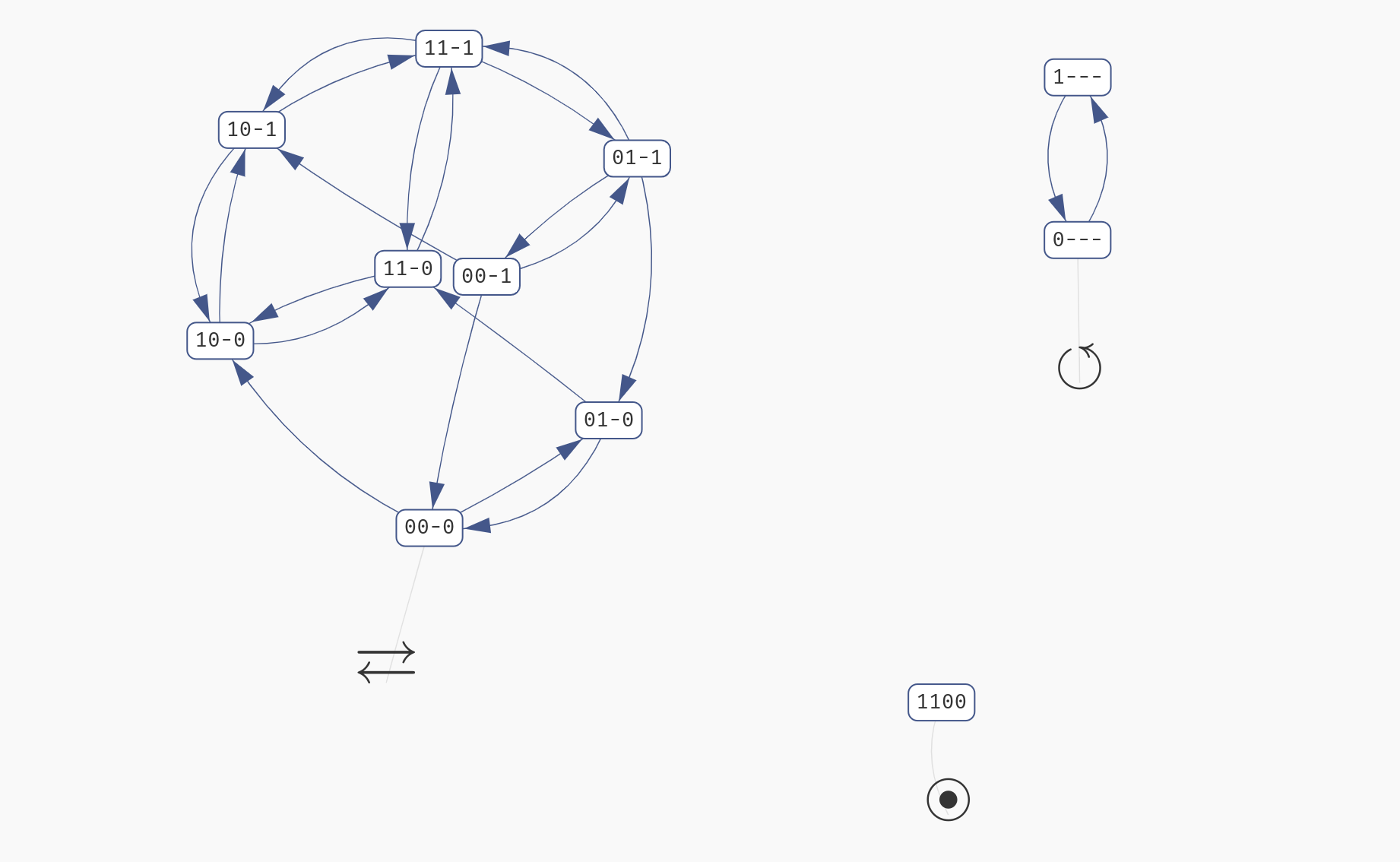
State space explorer
If you click the Attractors button in the Results panel, a state space explorer appears with the exact representation of the attractors discovered in the network for that particular behaviour class.
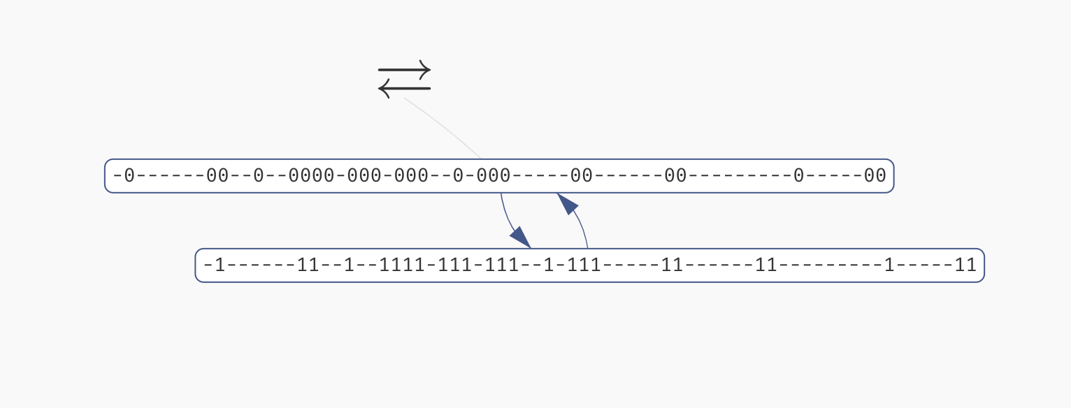
You can click each state to see a breakdown of the variables which are true (green) or false (red) in said state. In an oscillating or disordered attractor, the state labels will contain a dash (-) in place of variables which have a fixed (stable) value in the whole attractor. They will be also shown as grey in the variable values list. This way, you can quickly visually distinguish which variables are fixed and which are being updated in the attractor.
However, if your network is parametrised, remember that this visualisation always shows attractors of a fully specified Boolean network that was picked from the particular behaviour class. That is, state space of attractors in other parametrisations can be different. To show the update functions used in this particular network, you can click the Function button in the top left.
 Exploring the states of a disordered attractor.
Keep in mind that in a large network, you can use the
Find...functionality of your browser to quickly highlight the important variables in the list of variable values.
Finally, if the attractor is very large (approx. >5.000 states), we can't easily display it in a browser. We thus only show a simplified view of the attractor compressed into two states. In these two states, the stable variables have the values with which they appear in the attractor, and the unstable values simply all switch between true and false in one transition:
 A view of a large compressed attractor.
Bifurcation decision trees
To follow along with this section, you can download the .aeon model we will be using here. After loading it into AEON, you should see that the model has 66 variables and 13 parameters. Here, the parameters correspond to the input nodes of the regulatory graph, i.e. variables with no incoming regulations. Computing attractors for this model should take somewhere between 30 and 60 seconds.
The model can exhibit two behaviour classes: One with a stable attractor, and one with a disordered attractor. However, it is not clear which conditions lead to these two different classes! To explore this further, open the Bifurcation Function Explorer.
In this window, we will be constructing a bifurcation decision tree which describes how parameters alter the behaviour of the network. This decision tree consists of three types of nodes:
- A leaf node corresponds to a set of parametrisations which admit only a single behaviour class.
- A mixed node corresponds to a set of parametrisations which admit multiple behaviour classes.
- A decision node splits the parametrisations based on a value of a specific parameter.
Our goal will be to gradually turn mixed nodes into leaf or decision nodes to uncover which parameters influence the presence of different attractors in the network.
Initially, the tree contains a single mixed node with all admissible parametrisations of the network. By clicking the node, we reveal an overview similar to the Results panel in the main AEON window. However, we can also turn this mixed node into a decision node using the Make Decision button. This button will cause AEON to compute possible impact of picking different parameters as decision attributes. You will then be presented with a list of attributes (i.e. parameters) that you can use to split the mixed node into two. For each decision attribute, AEON shows you the impact of that decision on the behavior classes in the mixed node. If the decision isolates one behaviour class from the rest, a leaf node with that class will appear. Otherwise, a new mixed node is created.
 Creating decision nodes. Here, a parameter
 sigA is selected as the decision attribute, creating one leaf node with only disordered attractors, and one mixed node.
AEON will automatically sort the attributes based on how likely it is that they lead to a concise decision tree. We use information gain as the primary sorting criterion. However, you can also pick from other sorting heuristics:
- Total number of behaviour classes in both branches after making the decision.
- Number of parametrisations in the positive or negative branch.
- Number of parametrisations in the largest class (majority) of the positive/negative branch.
- Alphabetical sort.
There is generally no "best" decision attribute. The attribute you select usually depends on what you are trying to achieve with your decision tree. On the one hand, if you already have experimental data that you are trying to reproduce, you may be restricted to a set of measured/controllable parameters. On the other hand, if you are trying to explain the presence of a particular behaviour class, you may want to minimise the number of decisions necessary to isolate said class. And so on.
In our case, AEON will suggest glucose as the next decision attribute, producing the following tree:
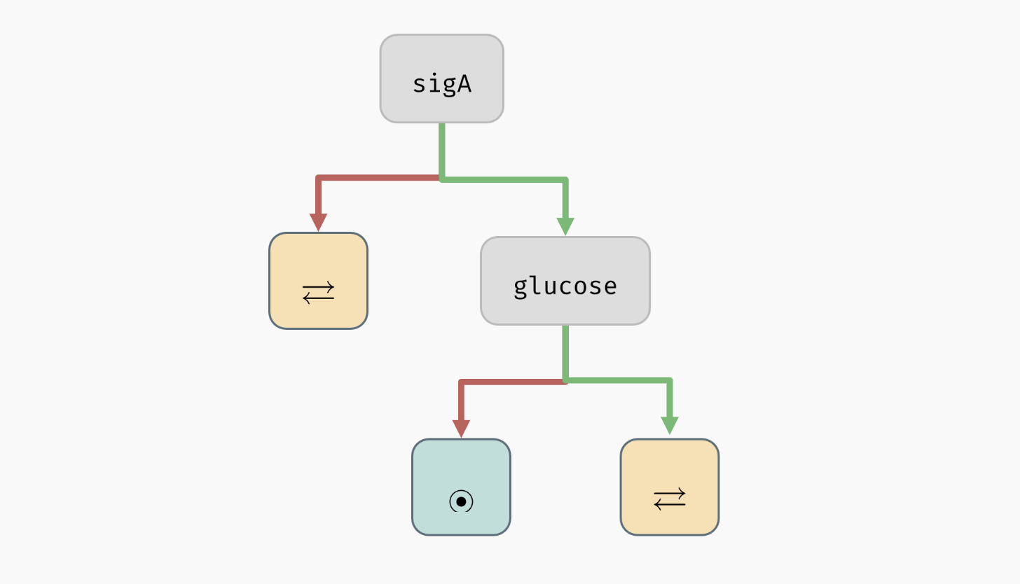 A decision tree for the example model.
As you can see, all mixed nodes are now gone. This is interesting, because as you may recall, the network has 13 parameters in total. However, only two of these parameters seem to actually play a role in the type of attractors appearing in the network (the remaining parameters can still determine what specific values the network variables take in the attractors -- we will explore this in the section about stability analysis). Furthermore, we can also clearly see that to bring the network into a stable state, it is sufficient to set sigA=true and glucose=false.
If you want to, you can now delete the decision nodes (select a node and click a red
Xin its corner) and try a different combination of decision attributes. You should discover that for this particular model, the remaining parameters indeed play no role in determining the attractor types: you will eventually have to make decisions onsigAandglucosein either case.
You can also generate a Witness network and explore Attractor state space for each leaf node of the tree, just as you could in the overview table of the bifurcation function. Furthermore, you can ask AEON to automatically expand a mixed node up to a certain depth using the Auto Expand function (AEON will use information gain to select the decision attributes).
Decision attributes of unknown Boolean functions
As you may have noticed, up to this point, the parameters of the network were always constants that can be either true or false, so it was simple to make decision nodes. If a network contains an uninterpreted function as a parameter (for example, recall the C | f(A, B) we used in the section about parametrised networks), it is not very clear how such a function can appear in a decision tree.
One option is to simply decide based on specific values in the function table. For example, f(0,1) could be a decision attribute that fixes the value of f(0,1) to be either true or false. However, it is often very hard to understand how a decision tree with such attributes translates to real life conditions. Specifically, if we want to test such condition in the real world, we would have to ensure that both inputs of the function are fixed to a specific value, which may not be always possible.
We thus also admit a different type of decision attributes for these parameters. We say that an input X is essential in function f if the value of f depends on the value of X (recall the observability property in regulatory graphs). We can then generalize this property further, and say that X is essential in f when Y=true. This means that not only f has to depend on the value of X, it has to depend on it when Y=true.
This kind of property should be easier to test and understand, because (a) we are only fixing a partial context (Y=true) for the function, instead of the entire input vector, and (b) we are clearly stating a variable (X) that is significant in determining the resulting value of the function in that context.
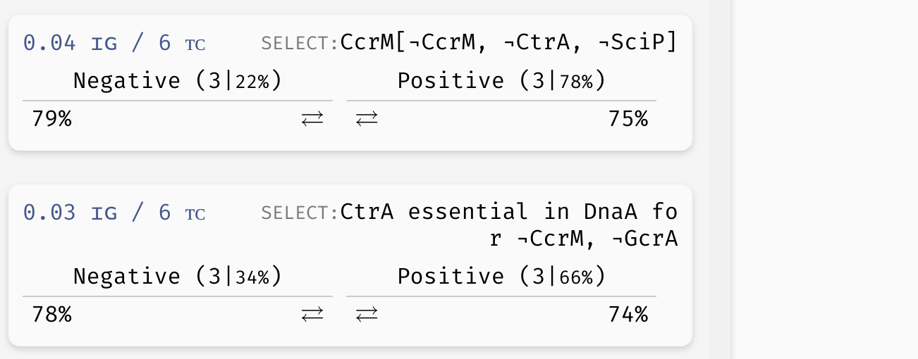 Example of a basic uninterpreted function constraint (implicitly parametrised function of variable
 CcrM is true for CcrM=CtrA=SciP=false), as well as an essentiality constraint (variable CtrA influences the outcome of the implicit function of DnaA when CcrM=GcrA=false).
To see these attributes in action, you can explore the decision tree of the model which we will now use to discuss trees with reduced precision...
Reduced precision trees
In some cases, the decision tree is not very concise and can be hard to read. For example, let's consider another version of the G2A model available here. This model is highly parametrised (in a rather unrealistic way nonetheless), and as a result, its bifurcation decision tree is quite large. However, in a lot of its nodes, there is a distinctive majority behaviour class that appears significantly more often than other classes.
In practice, we may want to allow a node with such a class to be regarded as a leaf, thus eliminating the remaining edge cases from the tree. In the bottom right corner of the AEON interface, you should see a Precision slider. By adjusting this slider, you specify what percentage of parametrisations needs to fall into a single class for a node to be accepted as a leaf. By default, this is set to the "exact" precision of 100%, however, you can reduce the number to collapse less likely branches of the tree into leaves:
 Collapsing branches of a complex tree with more than 90% majority behaviour class into leaves.
In a highly parametrised model, this is a great tool for focusing only on the most statistically significant types of behaviour.
Stability analysis
In many real world situations, what we are truly interested in is not only the type of attractor (stability, oscillation, disorder), but also the values of some significant variables in that attractor. In particular, in an attractor, a variable can be stable (always true, or always false) or unstable (changing its value depending on the attractor state). Recall that in the section about state space visualisation, we saw a disordered attractor with three unstable variables (v_1, v_2, and v_4), and one stable variable (v_3). In the presence of multiple attractors, we also say that a variable may exhibit switched behaviour if there are multiple attractors such that the stability properties of the variable change from attractor to attractor.
All these properties can change with respect to parameters, but don't alter the attractor type. To analyse these types of situations, AEON contains a Stability Analysis functionality which can further divide the parameter space based on the stability of individual variables.
You can run stability analysis for any node of the bifurcation decision tree (even mixed or decision nodes). This way, you can quickly assess how the stability of variables changes in your tree. Furthermore, you can also restrict the analysis based on the attractor type to only show how the variables change in these particular attractors. Finally, for each case, you can generate a Witness network as well as visualise the Attractor state space.
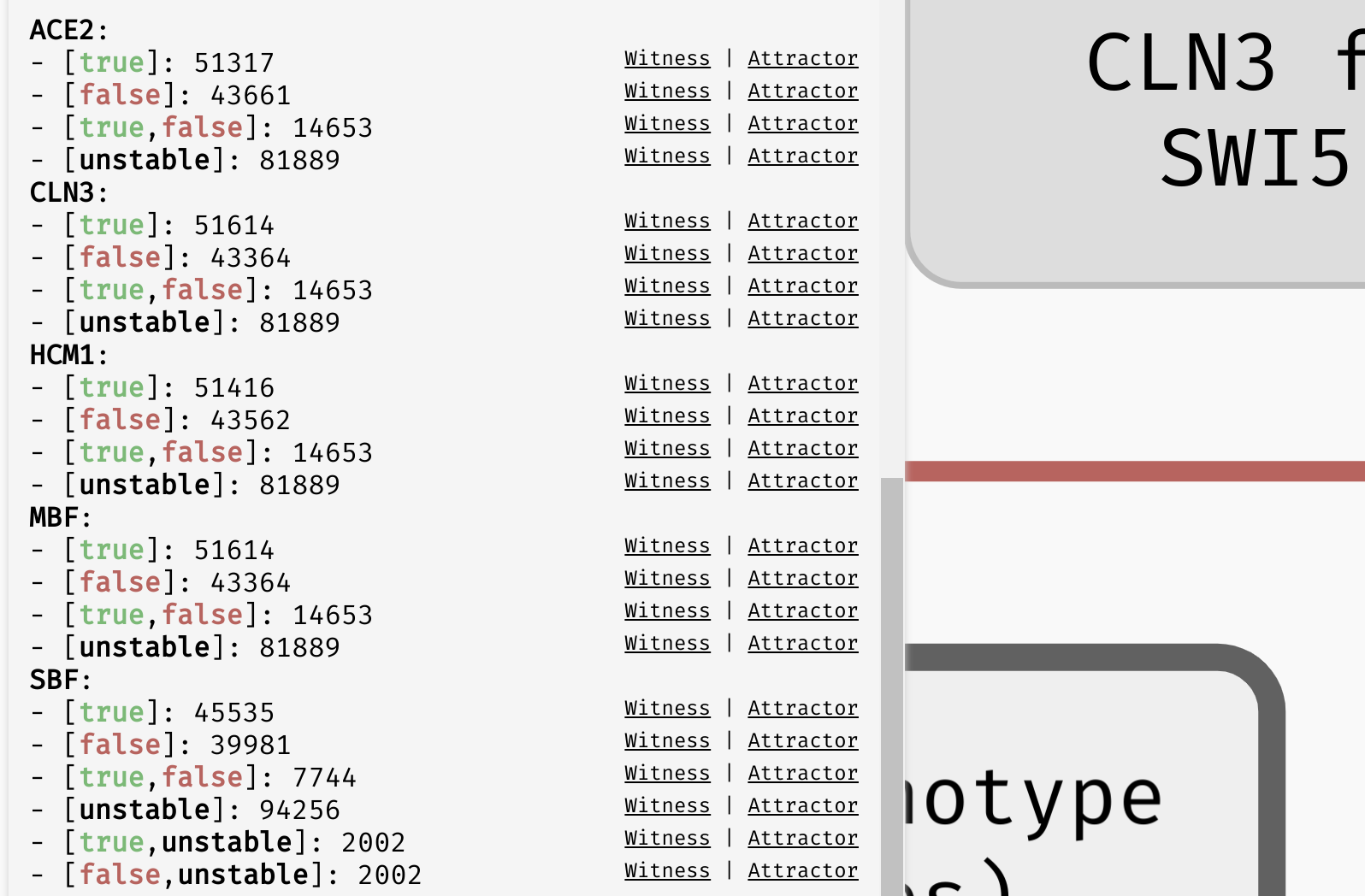 Stability analysis result for the
 Orlando example model. [true]/[false]/[unstable] represent situations where the variable always exhibits one type of behaviour, while multiple values (e.g. [true,false] or [true,unstable]) represent a switching behaviour.
Computation of Control
This section explains how to compute effective perturbations for controlling Boolean networks using Aeon.
What is Control in Boolean Networks?
Control in Boolean networks refers to the process of guiding the network toward a specific attractor, known as the phenotype. A phenotype represents a target state of the network, defined by a subset of variables assigned specific Boolean values.
To achieve this control, the network requires perturbations—sets of variables that are fixed to particular Boolean values. These perturbations ensure that the network's dynamics stabilize in the desired phenotype.
Aeon provides functionality to compute such perturbations, supporting permanent control, where selected variables remain fixed indefinitely. Once applied, these perturbations guarantee convergence of the network toward the target phenotype.
Interpretations of the Boolean Network
In this section, we use the term interpretation of the Boolean network/model. This term refers to different fully specified versions of the Boolean network. It is equivalent to the concept of a witness in attractor bifurcation.
The following sections will cover how to compute perturbations and analyze computed perturbations using Aeon’s visualization tools.
Task Settings for Control Computation
This section explains how to configure the necessary settings for computing control in Aeon. Specifically, we cover Control-Enabled status of variables and phenotype definition. Additionally, we discuss ways to refine control computation to obtain only the most relevant results and potentially speed up the process.
Control-Enabled status of Variables
Control-Enabled status determines whether a variable can be included in computed perturbations. Only variables explicitly marked as Control-Enabled may appear in perturbations. If a variable is Not-Control-Enabled, it remains unaffected by the control process.
Phenotype
A phenotype is the target state of the Boolean network, defined by a subset of variables assigned specific Boolean values. Control aims to drive the network toward this state, ensuring that once reached, it remains stable.
Additionally, Aeon distinguishes between oscillating and non-oscillating phenotypes. In a non-oscillating phenotype, the network stabilizes in the target state indefinitely. In contrast, an oscillating phenotype allows the network to transition cyclically through a set of states that include the desired phenotype. Aeon supports both types, enabling the analysis and control of networks with stable or dynamic target states.
Control-Enabled Editor
Aeon provides a dedicated editor for managing the Control-Enabled status of variables. This editor can be accessed by clicking the corresponding button in the left panel.
The primary purpose of the Control-Enabled Editor is to allow users to modify the Control-Enabled status of multiple variables simultaneously. Users can select variables from the table in the bottom section of the editor and toggle their Control-Enabled status. Only variables marked as Control-Enabled can be used in perturbations during the control computation process.
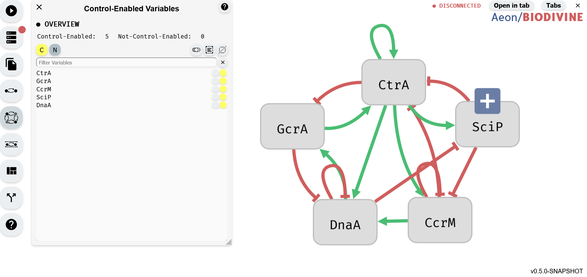 Control-Enabled Editor module (left) with regulatory graph editor (right)
Control-Enabled status Buttons
 Buttons for setting selected variables to Control-Enabled (left) and button for setting variables to Not-Control-Enabled (right)
Aeon provides two buttons for adjusting the Control-Enabled status of variables. Each button corresponds to a specific Control-Enabled status:
- The yellow button sets selected variables to Control-Enabled.
- The gray button sets selected variables to Not-Control-Enabled.
Clicking one of these buttons updates the Control-Enabled status of all variables currently selected in the Variable Editor.
Selection buttons
 Button to toggle selected variables (left), select all variables (center), and deselect all variables (right)
The Selection Buttons provide tools for efficiently selecting multiple variables in the Control-Enabled Editor. There are three buttons, each serving a different selection function:
- Toggle Selection (left, toggle switch icon) – Inverts the current selection: selected variables become unselected, and unselected variables become selected.
- Select All (center, square with lines icon) – Selects all variables in the editor.
- Deselect All (right, crossed-out square icon) – Clears the current selection, leaving no variables selected.
These buttons apply only to unfiltered variables. For example when a Variable Filter is applied, selecting all variables will select only those visible in the filtered list, leaving hidden variables unchanged.
Variable Filter
 Input for the varialbe filter
The Variable Filter is a text-based tool used to filter variables in the Control-Enabled Editor by name. The filter is case-sensitive and allows multiple variables to be filtered by separating their names with commas (,). It also supports partial matching, enabling searches for variables whose names start with a specific sequence of characters, even if incomplete.
Variable Table
The table at the bottom of the editor contains all the variables in the model. You can toggle the selection status of a variable by clicking on the corresponding row. To select or unselect multiple variables at once, hold down the left mouse button and drag over the variables. Selected variables are highlighted in blue.
Each row in the table displays the variable's name along with two circles:
- The circle on the right is the Control-Enabled status indicator. If it is yellow, the variable is Control-Enabled; if it is gray, the variable is Not-Control-Enabled.
- The circle on the left is the Add to Filter button, which adds the variable's name to the end of the Variable Filter.
Phenotype Editor
Aeon provides a dedicated editor for setting the phenotype of the control computation. This editor can be accessed by clicking the corresponding button in the left panel.
The primary purpose of the Phenotype Editor is to allow users to define the desired attractor of the network, specified as a set of variables with their desired Boolean values. Users can select variables from the table in the bottom section of the editor and assign them the appropriate values (true or false) to form the target phenotype. This phenotype will guide the control computation toward the desired attractor.
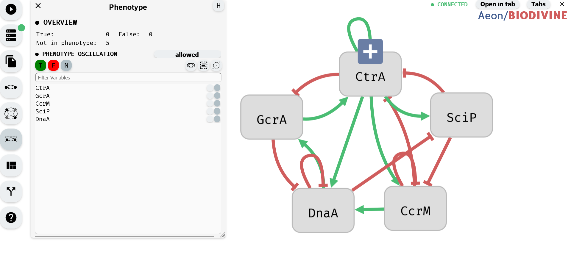 Phenotype Editor module (left) with regulatory graph editor (right)
Phenotype Oscillation
 Phenotype Oscillation Button
The Phenotype Oscillation button allows you to specify whether the perturbations should target an oscillating or non-oscillating phenotype. Phenotype oscillation occurs when the Boolean network alternates between being in the phenotype state and not being in it. If the phenotype is non-oscillating, the network will remain in the phenotype state indefinitely.
The button has three states:
- Allowed: Computes perturbations for both oscillating and non-oscillating phenotypes.
- Required: Computes perturbations only for oscillating phenotypes
- Forbidden: Computes perturbations only for non-oscillating phenotypes.
Phenotype Buttons
 Buttons for adding selected into phenotype as true (left), as false (middle) and button for removing selected variables from the phenotype (right)
Aeon provides three buttons for adjusting the phenotype of the model. Each button corresponds to a specific phenotype status:
- The green button adds the selected variables into the phenotype with a value of true.
- The red button adds the selected variables into the phenotype with a value of false.
- The gray button removes the selected variables from the phenotype.
Selection buttons
Button to toggle selected variables (left), select all variables (center), and deselect all variables (right)
The Selection Buttons provide tools for efficiently selecting multiple variables in the Control-Enabled Editor. There are three buttons, each serving a different selection function:
- Toggle Selection (left, toggle switch icon) – Inverts the current selection: selected variables become unselected, and unselected variables become selected.
- Select All (center, square with lines icon) – Selects all variables in the editor.
- Deselect All (right, crossed-out square icon) – Clears the current selection, leaving no variables selected.
These buttons apply only to unfiltered variables. For example when a Variable Filter is applied, selecting all variables will select only those visible in the filtered list, leaving hidden variables unchanged.
Variable Filter
Input for the varialbe filter
The Variable Filter is a text-based tool used to filter variables in the Control-Enabled Editor by name. The filter is case-sensitive and allows multiple variables to be filtered by separating their names with commas (,). It also supports partial matching, enabling searches for variables whose names start with a specific sequence of characters, even if incomplete.
Variable Table
The table at the bottom of the editor contains all the variables in the model. You can toggle the selection status of a variable by clicking on the corresponding row. To select or unselect multiple variables at once, hold down the left mouse button and drag over the variables. Selected variables are highlighted in blue.
Each row in the table displays the variable's name along with two circles:
- The circle on the right is the phenotype indicator. If it is green, the variable is in the phenotype as true; if it is red, the variable is in the phenotype as false; and if it is gray, the variable is not present in the phenotype.
- The circle on the left is the Add to Filter button, which adds the variable's name to the end of the Variable Filter.
Setting Control Settings with the Model Editor
In Aeon, some control settings can be modified not only through dedicated editors but also directly within the Model Editor. This functionality allows for quick adjustments to the Control-Enabled status and phenotype status of variables without switching to separate menus.
Each row in the Model Editor’s variable table includes two buttons, each corresponding to a specific control setting:
- Control-Enabled status Button – Toggles whether the variable is Control-Enabled.
- Phenotype Button – Adjusts the phenotype status of the variable.
Control-Enabled status Button
The Control-Enabled status Button is represented by a controller icon and is used to toggle the Control-Enabled status of a variable. Clicking on this button changes whether the variable can be included in perturbations. The button also visually indicates the variable's Control-Enabled status through its color:
- Yellow – The variable is Control-Enabled.
- Grey – The variable is Not-Control-Enabled.
 Making Control-Enabled variables Not-Control-Enabled using the Model Editor
Phenotype Button
The Phenotype Button is represented by a target icon and is used to modify the phenotype status of a variable. Clicking on this button toggles whether the variable is included in the phenotype and, if so, whether it is set to true or false. The button's color visually indicates the variable’s phenotype status:
- Green – The variable is included in the phenotype as true.
- Red – The variable is included in the phenotype as false.
- Gray – The variable is not included in the phenotype.
 Setting of the phenotype using the Model Editor
Limiting the Control Computation
Aeon provides options for restricting the control computation, allowing users to filter out redundant results and, in some cases, improve performance. These options can be found under the Control Computation Mode in the Start Computation module, accessible by clicking the corresponding button in the left panel.
 Navigation to the options for limiting the control computation
The available limiting settings include:
- Min Robustness (%) – The minimum percentage of Boolean network interpretations for which a computed perturbation must be effective. This is a real number with two decimal places, ranging from 0 to 100.
- Max Size – The maximum number of variables allowed in a perturbation. This is a whole number starting from 0. By default, it is set to the number of Control-Enabled variables in the model.
- Max Number of Results – The maximum number of perturbations to compute. This is a whole number starting from 0. The default value is set to 1,000,000.
Control Results
This section outlines the features Aeon provides for analyzing and managing the results of control computations. Aeon offers various visualization methods and export options to facilitate the interpretation and further use of computed perturbations.
Both visualization and export options are available in the Results module. This module opens automatically after a successful computation and can also be accessed by clicking the corresponding button in the left panel.
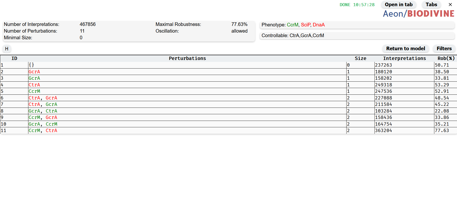
Perturbation Table
 Perturbation Table
The Perturbation Table provides a structured visualization of the perturbations computed during the control process. Each row in the table represents a single perturbation along with relevant details.
Format of Perturbations
By default, perturbations are displayed in a color-coded format, where variables included in the perturbation are highlighted based on their Boolean value:
- Green indicates the variable should be set to true.
- Red indicates the variable should be set to false.
 Perturbation Color Format
Alternatively, Aeon offers a text format for representing perturbations. In this format, each perturbation is listed with variable names followed by the Boolean value they should be fixed to, separated by a colon (:).
 Perturbation Text Format
You can toggle between these two formats for an individual perturbation by clicking on its visualization within the row. To switch the format for all perturbations at once, click on the Perturbation header of the table.
Details about Perturbation
 Perturbations with details about them
Each row in the table not only displays the perturbation itself but also provides additional relevant information:
- ID – A unique identifier for the perturbation.
- Size – The number of variables included in the perturbation.
- Interpretations – The number of Boolean network interpretations for which the perturbation is effective.
- Rob (%) – The robustness of the perturbation, expressed as a percentage. This indicates the proportion of network interpretations where the perturbation successfully achieves the desired control.
Filters and Sorts
Filters and sorts for the Perturbation table are accesible by clicking on the Filters button. You can hide them again by clicking the button or by clicking the cross in the left corner of the filters module.
 How to navigate to the Filter Menu and demonstration of basic filtering
Max Size
Maximal size Filters from the table perturbation which contain more than specified number of variables. Whole number from 0.
Min NoI
Minimal Number of Interpretations. Filters from the table perturbation which work for less than specified number of interpretations of the model. Whole number from 0.
Min Robustness (%)
Minimal Robustness. Filters from the table perturbations which work for less than specified % of models interpretations. a real number with two decimal places, ranging from 0 to 100.
Filter by Fixed Variables
 Filter by Fixed Variables
This filter allows specifying which variables should be included in the perturbation and with what Boolean values. To configure the filter:
- Select variables by clicking on them or using the Selection Buttons.
- Assign values using the Variable Perturbation Status Buttons.
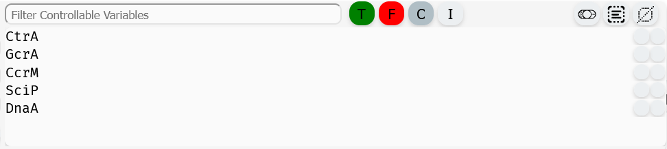
Variable Perturbation Status Buttons
 Variable Perturbation Status Buttons
These buttons define how selected variables should appear in the filtered perturbations:
- Green (T) – The variable must be true in the perturbation.
- Red (F) – The variable must be false in the perturbation.
- Gray (C) – The variable must be included in the perturbation, regardless of its value.
- Light Gray (I) – The variable is removed from the filter.
Clicking one of these buttons updates the filter status for all selected variables.
Selection buttons
 Button to toggle selected variables (left), select all variables (center), and deselect all variables (right)
The Selection Buttons provide tools for efficiently selecting multiple variables in the Control-Enabled Editor. There are three buttons, each serving a different selection function:
- Toggle Selection (left, toggle switch icon) – Inverts the current selection: selected variables become unselected, and unselected variables become selected.
- Select All (center, square with lines icon) – Selects all variables in the editor.
- Deselect All (right, crossed-out square icon) – Clears the current selection, leaving no variables selected.
These buttons apply only to unfiltered variables. For example when a Variable Filter is applied, selecting all variables will select only those visible in the filtered list, leaving hidden variables unchanged.
Variable Filter
 Input for the variable filter
The Variable Filter is a text-based tool used to filter variables in the table of the Fixed Variables filter by name. The filter is case-sensitive and allows multiple variables to be filtered by separating their names with commas (,). It also supports partial matching, enabling searches for variables whose names start with a specific sequence of characters, even if incomplete.
Variable Table
The Variable Table within the filter module lists all Control-Enabled variables in the model. Variables can be selected by clicking on their row or multi-selected by dragging the left mouse button over them. Selected variables are highlighted in blue.
Each row in the table contains the variable name and two indicator circles:
-
Filter Status Indicator (right circle) – Shows how the variable is included in the filter:
- Green – Variable is in the filter as true.
- Red – Variable is in the filter as false.
- Gray – Variable must be included in the perturbation, regardless of value.
- Light Gray – Variable is not included in the filter.
-
Add to Filter Button (left circle) – Adds the variable's name to the Variable Filter input field.
Sorting Options
Sorting in the Perturbation Table is controlled using two sorting widgets: Primary Sort (left) and Secondary Sort (right).
Each sorting widget consists of:
-
A sorting parameter button that determines the sorting criterion:
- ID – Sort by perturbation ID.
- Size – Sort by the number of variables in the perturbation.
- NoI (Number of Interpretations) – Sort by the number of model interpretations for which the perturbation is valid (equivalent to sorting by robustness).
-
A sorting order button that sets the sorting direction:
- Upward Arrow – Ascending order.
- Downward Arrow – Descending order.
Sorting Behavior:
- Primary Sort determines the main sorting order.
- Secondary Sort applies when multiple perturbations share the same value in the Primary Sort criterion.
- If the same parameter is selected for both sorts, the Secondary Sort has no effect.
- If the Primary Sort is set to "ID", the Secondary Sort is ignored, as IDs are always unique.
Export of Control Results
The export functionality in the Results module allows saving computed control results for further analysis and use outside Aeon. Currently, Aeon supports exporting results in the following formats:
CSV (.csv)
The CSV format provides a structured, tabular representation of the computed control perturbations, making it easy to process the data in spreadsheet applications or external analysis tools.
Control Computation Demonstration
This section provides a step-by-step guide for running an example control computation in Aeon. It covers the setup process, parameter configuration, and execution of the computation.
1. Running Aeon
 State of the Aeon tool at startup
Aeon can be accessed either through its online version ([URL]) or by downloading and running it locally ([URL]).
2. Connecting the Compute Engine
Open the Compute Engine module from the left panel to check the connection status. If the Compute Engine is not connected, download the appropriate version for the system from the bottom of the module and run it locally.
 Downloading AEON compute engine.
 Connecting to a running compute engine.
3. Importing or Creating a Model
A model can be created using the Model Editor or imported through the Import/Export module, both accessible from the left panel. The Import/Export module allows loading a model from local storage or selecting one of the default models available at the bottom of the module.
 Import of the G2A example model
4. Setting Control-Enabled Variables
The Control-Enabled Editor module, accessible from the left panel, is used to define which variables are Control-Enabled and can be included in perturbations. By default, variables are set as Control-Enabled unless specified otherwise in the imported model.
To change the Control-Enabled status of multiple variables, select them and use the Control-Enabled status Buttons.
 Making Control-Enabled variables Not-Control-Enabled using the Control-Enabled Editor
Alternatively, Control-Enabled status can be modified for individual variables using the Model Editor module.
 Making Control-Enabled variables Not-Control-Enabled using the Model Editor
5. Defining the Phenotype
The Phenotype Editor module, located in the left panel, is used to specify the phenotype of the model by assigning Boolean values to selected variables. By default, variables are not part of the phenotype unless specified in the imported model.
- To add variables to the phenotype as true, select them and click the green button.
- To add variables to the phenotype as false, select them and click the red button.
- To remove variables from the phenotype, select them and click the gray button.
 Setting of the phenotype using the Phenotype Editor
The Model Editor module can also be used to set phenotype values for individual variables.
 Setting of the phenotype using the Model Editor
6. Configuring Computation Limits and Starting the Process
In the Start Computation module, accessible from the left panel, set the computation mode to Control. Under the Control Settings section, configure computation limits:
- Min Robustness (%) – Minimum percentage of Boolean network interpretations for which perturbations must work.
- Max Size – Maximum number of variables allowed in a perturbation.
- Max Number of Results – Maximum number of computed perturbations.
Once parameters are set, start the computation using the button at the bottom of the module.
 Setting computation limits and starting the computation
7. Viewing Control Results
Once the computation is complete, the Results module opens automatically, displaying a summary of results. If needed, this module can also be accessed from the left panel.
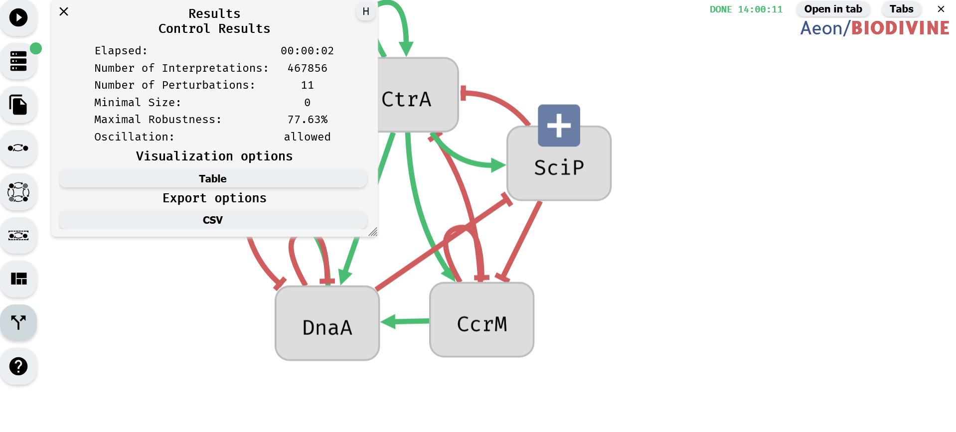 Control Results Module
The results can be further explored using visualization options or exported for external use.
Tab System
Aeon includes a tab system for managing multiple result visualizations efficiently. Each newly opened visualization appears as an inner tab, accessible through the Tab Menu. This system allows users to keep multiple visualizations open while working on the same model.
Tab Menu
The Tab Menu contains all opened visualizations related to the current model.
- Opening the Tab Menu – Click the Tabs button in the upper right corner of the tool.
- Hiding the Tab Menu – Click the Tabs button again to close it.
 Demonstration of the Inner Tab Menu
Opening Inner Tabs in a New Browser Tab
To open an inner tab in a separate browser tab, click the Open in Tab button, located to the left of the Tabs button.
 Opening inner tab with Perturbation Table in a new browser tab
Closing Inner Tabs
You can close an inner tab by clicking the X button in the upper right corner of the tab.
- This option is available only when more than one inner tab is open.
 Closing inner tab
Returning to the Model Tab
Certain visualizations include a Return to Model button.
Clicking this button switches to the model's inner tab. If the model's inner tab was previously closed, a new inner tab with the model will be opened.
Building Aeon
AEON lives in two Github repositories and is available under a permissive MIT license. First repository manages the web frontend, and the second one is responsible for the compute engine.
Deploying the web frontend
If you want to run your own version of the AEON frontend, you simply need to download the latest source files from the aeon-client repository (or download the sources for a particular release based on its tag). Then, you can either open the index.html file in your favourite browser, or deploy the whole directory to any webserver that is able to serve static content.
Compiling the compute engine
To run your own version of the compute engine, you need to download the source files from the aeon-server repository (again, you can either download the latest version from the master branch, or sources for a specific version based on its tag). To run or compile the compute engine, you will need the Rust nightly compiler. We recommend following the installation instructions on rust-lang.org. These will install the whole distribution into your local ~/.cargo folder, hence they do not require any elevated privileges (as opposed to some OS package managers).
Once you have completed the setup process, you need to switch from
stableto thenightlycompiler by executing:rustup default nightly
Once you have the compiler ready, you can navigate to the source files you downloaded from Github, and execute
cargo run --release
to immediately compile and start the compute engine. Alternatively, you can also run
cargo build --release
which will generate the compute engine binary in ./target/release/biodivine-aeon-server.
Building this manual
This manual is available in the aeon-server repository in the manual directory, and is managed using the mdBook tool. You can follow the instructions on their website to install mdbook. Once you have mdbook ready, you simply need to navigate to the manual folder and run mdbook build to write the output files into the book directory (from here, you can deploy them as a static website). Alternatively, you can run mdbook serve to open a local webserver at http://localhost:3000 which serves the manual from your machine and automatically updates when you change its contents.